pacman::p_load(tmap,sf,tidyverse)In-class Exercise 1: My first date with Geospatial Data Analytics.
Getting started
The code chunk below load the following packages:
tmap: for thematic mapping
sf: for geospatial data handling
tidyverse: for non-spatial data handling
Preparing the Flow data
Importing the OD data
Firstly, we will import the Passenger Volume by Origin Destination data set downloaded from LTA DataMall by using read_csv() of readr package.
odbus <-read_csv("data/aspatial/origin_destination_bus_202308.csv")A quick check of odbus tibble data frame
odbus$ORIGIN_PT_CODE<-as.factor(odbus$ORIGIN_PT_CODE)
odbus$DESTINATION_PT_CODE<-as.factor(odbus$DESTINATION_PT_CODE)
Extracting the study data
For the purpose of this exercise, we will extract commuting flows on weekday and between 7 and 9 o’clock
origin7_9<-odbus %>%
  filter(DAY_TYPE == "WEEKDAY") %>%
  filter(TIME_PER_HOUR >= 7 &
           TIME_PER_HOUR <= 9) %>%
  group_by(ORIGIN_PT_CODE) %>%
  summarise(TRIPS = sum(TOTAL_TRIPS))
busstop <- st_read(dsn = "data/geospatial", layer = "BusStop")%>%
st_transform(crs=3414)Reading layer `BusStop' from data source
`C:\Users\Lian Khye\Desktop\MITB\Geospatial\geartooth\ISSS624\In-class_Ex\Ex1\data\geospatial'
using driver `ESRI Shapefile'
Simple feature collection with 5161 features and 3 fields
Geometry type: POINT
Dimension: XY
Bounding box: xmin: 3970.122 ymin: 26482.1 xmax: 48284.56 ymax: 52983.82
Projected CRS: SVY21mpsz <- st_read(dsn = "data/geospatial", layer = "MPSZ-2019") %>%
st_transform(crs=3414)Reading layer `MPSZ-2019' from data source
`C:\Users\Lian Khye\Desktop\MITB\Geospatial\geartooth\ISSS624\In-class_Ex\Ex1\data\geospatial'
using driver `ESRI Shapefile'
Simple feature collection with 332 features and 6 fields
Geometry type: MULTIPOLYGON
Dimension: XY
Bounding box: xmin: 103.6057 ymin: 1.158699 xmax: 104.0885 ymax: 1.470775
Geodetic CRS: WGS 84mpszSimple feature collection with 332 features and 6 fields
Geometry type: MULTIPOLYGON
Dimension: XY
Bounding box: xmin: 2667.538 ymin: 15748.72 xmax: 56396.44 ymax: 50256.33
Projected CRS: SVY21 / Singapore TM
First 10 features:
SUBZONE_N SUBZONE_C PLN_AREA_N PLN_AREA_C REGION_N
1 MARINA EAST MESZ01 MARINA EAST ME CENTRAL REGION
2 INSTITUTION HILL RVSZ05 RIVER VALLEY RV CENTRAL REGION
3 ROBERTSON QUAY SRSZ01 SINGAPORE RIVER SR CENTRAL REGION
4 JURONG ISLAND AND BUKOM WISZ01 WESTERN ISLANDS WI WEST REGION
5 FORT CANNING MUSZ02 MUSEUM MU CENTRAL REGION
6 MARINA EAST (MP) MPSZ05 MARINE PARADE MP CENTRAL REGION
7 SUDONG WISZ03 WESTERN ISLANDS WI WEST REGION
8 SEMAKAU WISZ02 WESTERN ISLANDS WI WEST REGION
9 SOUTHERN GROUP SISZ02 SOUTHERN ISLANDS SI CENTRAL REGION
10 SENTOSA SISZ01 SOUTHERN ISLANDS SI CENTRAL REGION
REGION_C geometry
1 CR MULTIPOLYGON (((33222.98 29...
2 CR MULTIPOLYGON (((28481.45 30...
3 CR MULTIPOLYGON (((28087.34 30...
4 WR MULTIPOLYGON (((14557.7 304...
5 CR MULTIPOLYGON (((29542.53 31...
6 CR MULTIPOLYGON (((35279.55 30...
7 WR MULTIPOLYGON (((15772.59 21...
8 WR MULTIPOLYGON (((19843.41 21...
9 CR MULTIPOLYGON (((30870.53 22...
10 CR MULTIPOLYGON (((26879.04 26...busstop_mpsz <- st_intersection(busstop, mpsz) %>%
select(BUS_STOP_N, SUBZONE_C) %>%
st_drop_geometry()origin_SZ <- left_join(origin7_9 , busstop_mpsz,
by = c("ORIGIN_PT_CODE" = "BUS_STOP_N")) %>%
rename(ORIGIN_BS = ORIGIN_PT_CODE,
ORIGIN_SZ = SUBZONE_C) %>%
group_by(ORIGIN_SZ) %>%
summarise(TOT_TRIPS = sum(TRIPS))origintrip_SZ <- left_join(mpsz,
origin_SZ,
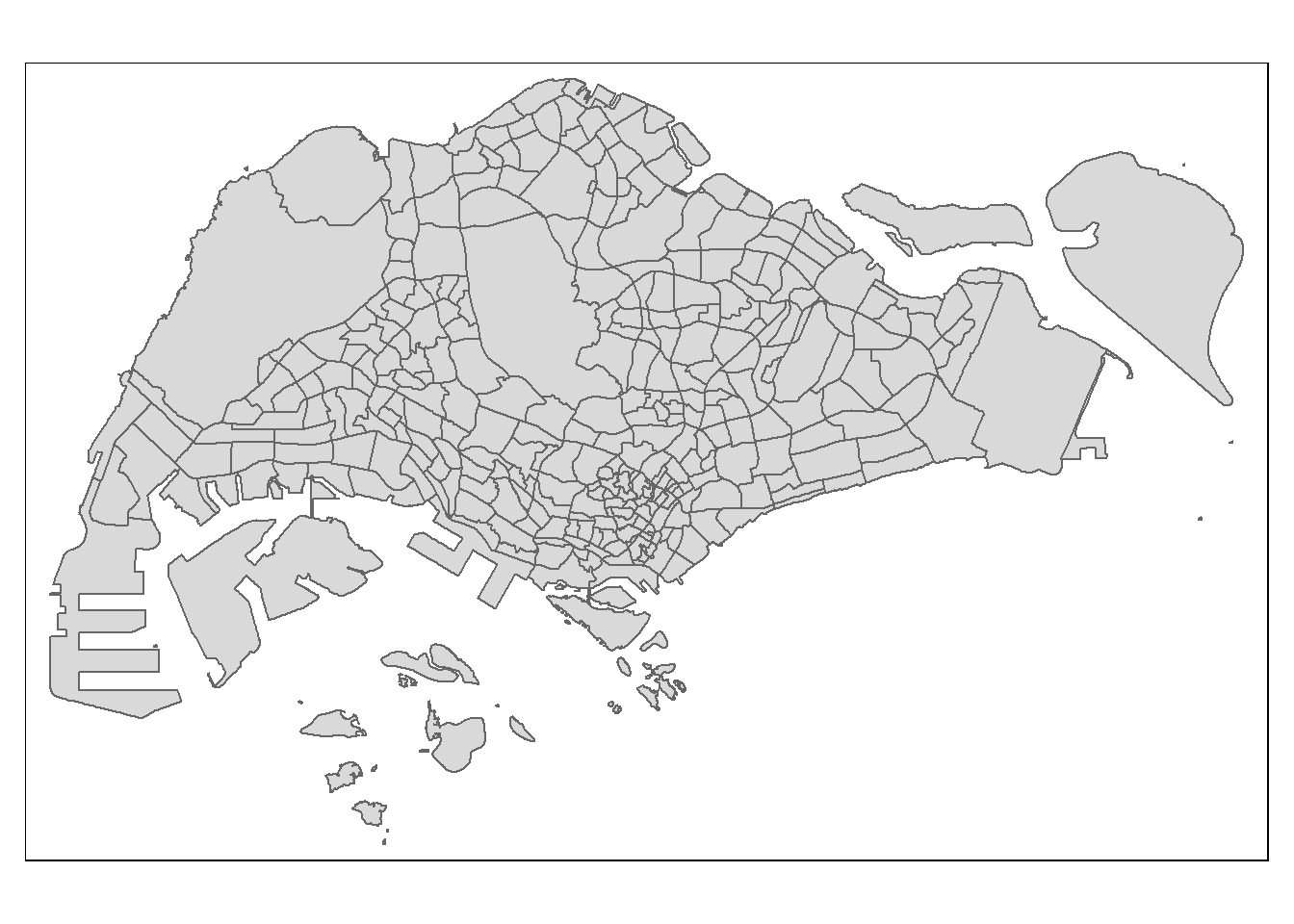
by = c("SUBZONE_C" = "ORIGIN_SZ"))basemap <- tm_shape(origintrip_SZ) +
tm_polygons()
basemap